3 Methods

3.1 General Analysis Pipeline of Bulk RNA-Seq Data

The analysis pipeline used to process the bulk RNA-Seq data of both in-houses and downloaded datasets, is shown in Figure 3.1. Briefly, the analysis of RNA-Seq started with assessing the quality of raw sequencing data as fastq files using FASTQC (v0.11.4). Once the quality was deemed fit for further processing, the fastq files were mapped to GRCh38/hg38 using HISAT2 (v2.1.0), resulting in BAM files. The coordinate sorted BAM files were then indexed using SAMTOOLS (v1.9). The number of reads assigned to each feature of the genome was estimated using FeatureCounts of SUBREAD module (v1.6.3) with Homo_sapiens.GRCh38.96.chr.gtf as the reference genome .gtf file. The alignment, indexing and abundance estimation were performed on the GWDG-high performance computing (HPC) cluster. Count text files were imported into R (v3.6.1) running under macOS Mojave 10.14.5 for further processing. The data was normalized to either Z-scale or variable stabilized normalization in R using the DESeq2 package’s (v1.25.10) vst() function. PCA plots were made using R’s base function prcomp(). The visualization was performed using the ggplot2 package (v3.2.1). Several other packages and few custom functions were used throughout this project. The bash and R scripts can be found here, along with the output from sessionInfo() from R.

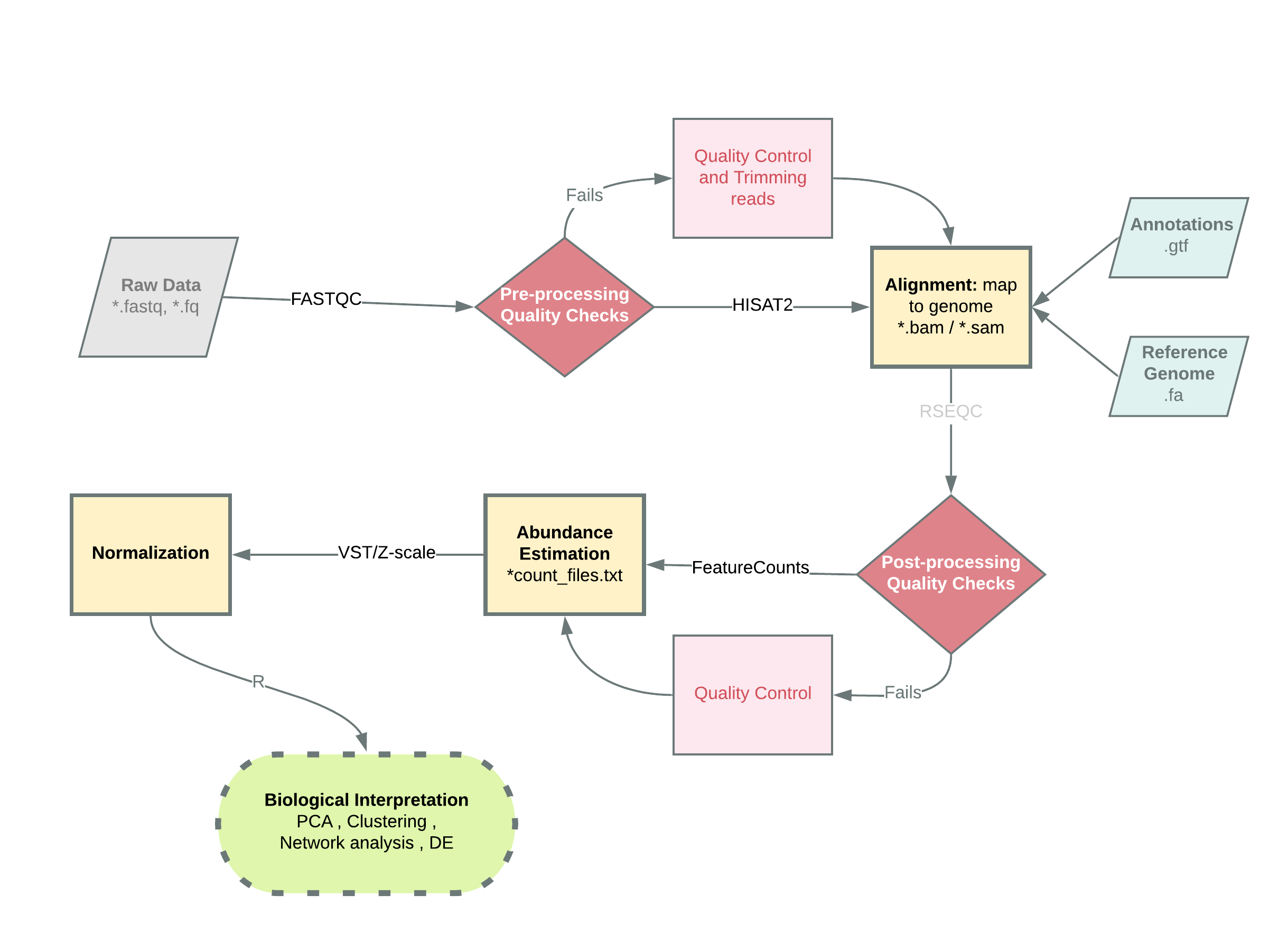
Figure 3.1: Basic analysis pipeline for Bulk RNA-Seq data used in this project. Briefly, raw sequenced data input as fastq files are run through FASTQC for basic quality checks, after which depending on the quality it either goes through additional steps of quality control or directly to an alignment tool like that of HISAT2. An optional post-alignment, quality control check exists, after which abundance of the transcripts is estimated using a tool such as FeatureCounts. This gived the raw read counts file which needs to then be normalized and then used for further analysis. Shapes and their meanings: Parallelograms (inputs), rhombus (decision points), rectangles (processes), oval (termination). Abbreviation: VST (variance stabilized transformation), PCA (principal component analysis), .fastq/.fa./fq (raw reads file format), .bam/.sam (binary alignment map, sequence alignment map – file formats for storing aligned sequence data), .gtf (gene transfer format – stores information on genes) .

The bulk RNA-Seq data used in this project is collated from different sources, which are tabulated in table 3.1 along with their accession numbers and the numbers of samples^59–63.

Table 3.1: blah blah

paper	Project_AccessionNumber	group	n
In-House	In-House	CM	20
In-House	In-House	EHM	10
In-House	In-House	Fetal_Heart	3
In-House	In-House	Fib	4
In-House	In-House	ipsc	2
In-House	In-House	Rh	2
Kuppusamy KT 2015	PRJNA266045	Adult_Heart	2
Kuppusamy KT 2015	PRJNA266045	Fetal_Heart	2
Mills RJ 2017	PRJNA362579	Adult_Heart	1
Mills RJ 2017	PRJNA362579	EHM	7
Pavlovic BJ 2018	PRJNA433831	Adult_Heart	12
Pervolaraki 2018	E_MTAB_7031	Fetal_Heart	9
Yan L 2016	PRJNA268504	Fetal_Heart	2
Note:
CM: cardiomyocytes, EHM: engineered heart muscle, Fib: iPSC-induced fibroblasts, Rh: rhesus iPSC-induced cardiomyocytes

3.2 Single Cell Reference Data and CIBERSORTX

Efficient deconvolution of bulk data requires a relevant single cell reference to estimate proportions of different cell types. For the current work we used reference data obtained by Friedman et al⁵⁸ who investigated cardiac differentiation of human pluripoten stem cells and performed single-cell transcriptomic analyses to map fate changes and analyze gene expression patterns during the differentation processes in vitro. In this approach 5 distinct time points were sequenced, namely, on days 0 (hiPSC), 2 (germ layer specification), 5 (progenitor cell), 15 (committed cardiac derivative) and 30 (definitive cardiac derivative) of their differentiation protocol. Relevant to this project are the last two timepoints — day 15 and day 30. Single-cell count data was downloaded from the ArrayExpress database maintained by EMBL-EBI, using the accession number E-MTAB-6268.
CIBERSORTX⁴⁷ reads a single cell reference input with each single-cell (every column) labelled according to the cell’s phenotype or cluster identifier and bulk data with samples as columns and rownames as genes in both cases.

3.2.1 Processing of Single Cell Data

To create the reference file, clustering and de novo identification of cell types from scRNA data was performed according to Friedman et al’s paper⁵⁸. Briefly, the outlier genes and cells (outside 3x median absolute deviation) of the number of cells with detected genes, mitochondrial reads, ribosomal genes were filtered out. Post filtering, scran (1.12.1) package was used for cell-to-cell normalization without quickClustering option. PCA and clustering was performed using ascend package (v0.9.93), following the same parameters as the paper.

The differentially expressed genes between the clusters were then calculated by the runDiffExpression() from ascend package. Friedman et al identified two clusters at each of the last two time points. At Day 15, they define two sub-populations — non-contractile (d15:S1) and committed CM (cCM) (d15:S2) and likewise at Day 30 — non-contractile (d30:S1) and definitive CM (dCM) (d30:S2). To verfiy the steps followed so far and validate the reliable reproduction of the paper, gene ontology analysis of differentially expressed genes within the sub clusters was performed. Figure 3.2 confirms that the clusters are consistent with the ones described by Friedman et al.

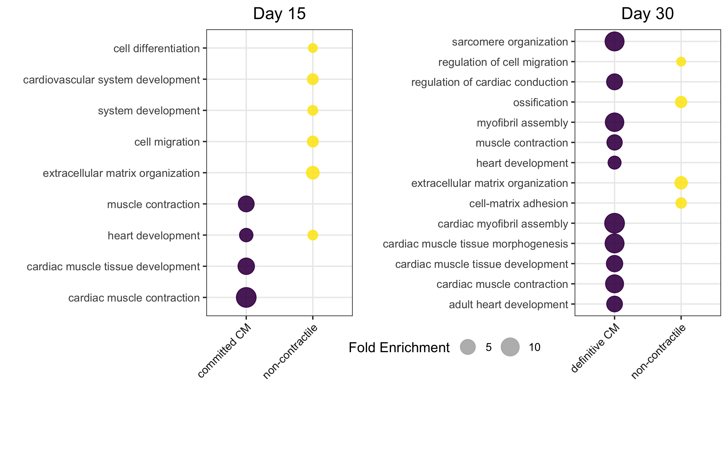
Figure 3.2: scRNA-Seq Reference Dataset. Post-processing and before feeding it into CIBERSORTx, the reference data set was analyzed to ensure its reliable reproduction of the sub-groups as defined by the paper. Here, at both time points there is a sub-group which is enriched for non-contractile features and another for cardiomyocyte features. The size of the circle corresponds to the fold enrichment observed. Reproduction of Figure 2 (J and M) from Friedman 2018.

CIBERSORTX is an online tool with user-friendly GUI with detailed tutorials on the developer’s webpage. Firstly, a signature matrix was created using this single cell reference file using the Create Signature Matrix function using scRNA-Seq as the input data type and all other settings were left at default. In the second step of deconvolution analysis, mode is set to Impute Cell Fractions and under Custom mode, the previously run signature matrix file is chosen from the drop down menu and a mixture file, previously uploaded bulk RNA-Seq data, is chosen. The option enable batch correction was used with B-Mode, which is advised for removing technical differences between the platforms used for the signature and bulk matrices. Finally, for the permutations for significance analysis option, the most stringent, 1000 option was chosen.

3.3 Analysis of Rhesus RNA-Seq

The bulk in-house samples from Rhesus were mapped using HISAT2 with default parameters. There was no indexed reference genome readily available, so the entire genome was downloaded in from USCS Genome Browser — rheMac10 assembly and converted from 2bit format to Fasta format using twoBitToFa available at USCS. Post alignment, abundance estimation was performed using the FeatureCounts tool which requires a valid .gtf file. The file was prepared using the following commands:

#Download

wget -c -O mm9.refGene.txt.gz filePathLinked

#Unzip the file and download the genePredToGtf tool from ucsc

cut -f 2- rheMac10.refGene.txt > refGene.input

./genePredToGtf file refGene.input rheMac10refGene.gtf

cat rheMac10refGene.gtf | sort -k1,1 -k4,4n > rheMac10refGene.gtf.sorted

This rheMac10refGene.gtf.sorted file was used as the input .gtf file for FeatureCounts. This outputs the raw counts file of the Rhesus macaque sample mapped to it’s own genome. To make comparisons with the human RNA-Seq samples relevant, orthologous genes between the two species were determined and only those with 1:1 orthology were used for further analysis. Orthologous genes were obtained from ensembl-biomart. The gene lengths of each gene was used for both species as a means of normalization within DESEQ2 by adding a matrix of gene lengths within the assays(dds)[["avgTxLength"]] <- geneLengthMatrix slot.

3.4 Estimating Bacterial and Viral Contaminants

DecontaMiner⁶⁴ was used to estimate the possible bacterial and viral contaminants in a representative subset of bulk samples of this project. Briefly, the unmapped reads i.e., those that failed to map to the reference genome were collected in a separate directory and mapped to bacterial and viral reads using the genome databases (NCBI nt) using MegaBLAST algorithm, specifying the number of allowed mismatches/gaps and the alignment length. The BLAST databases have been curated by downloading the sequences of the complete genomes from the RefSeq repository. These .fasta files were assembled into blast databases by running the makeblastdb command. Files containing discarded reads along the pipeline are also generated — the low quality ones, ones mapped to mtRNA/rRNA and ambiguous and unaligned reads. The second part of the pipeline, involves setting a match count threshold (MCT) — minimum number of reads successfully mapped to a single organism to consider it a contaminant. This parameter was set at 100 (default is 5). The pipeline once run results in a table containing all the matches satisfying the alignment criteria.

References

47. Newman, A. M. et al. Determining cell type abundance and expression from bulk tissues with digital cytometry. Nature Biotechnology 37, 773–782 (2019).

58. Friedman, C. E. et al. Single-Cell Transcriptomic Analysis of Cardiac Differentiation from Human PSCs Reveals HOPX-Dependent Cardiomyocyte Maturation. Cell Stem Cell 23, 586–598.e8 (2018).

59. Kuppusamy, K. T. et al. Let-7 family of microRNA is required for maturation and adult-like metabolism in stem cell-derived cardiomyocytes. Proceedings of the National Academy of Sciences of the United States of America 112, E2785–2794 (2015).

63. Yan, L. et al. Epigenomic Landscape of Human Fetal Brain, Heart, and Liver. The Journal of Biological Chemistry 291, 4386–4398 (2016).

64. Sangiovanni, M., Granata, I., Thind, A. S. & Guarracino, M. R. From trash to treasure: Detecting unexpected contamination in unmapped NGS data. BMC Bioinformatics 20, 168 (2019).