4 Results and Discussion

4.1 General Workflow and Mapping Statistics

Given that the analysis of RNA-Seq data is multi-faceted with distinct steps, a common work-flow modality was established as shown in Figure 4.1.

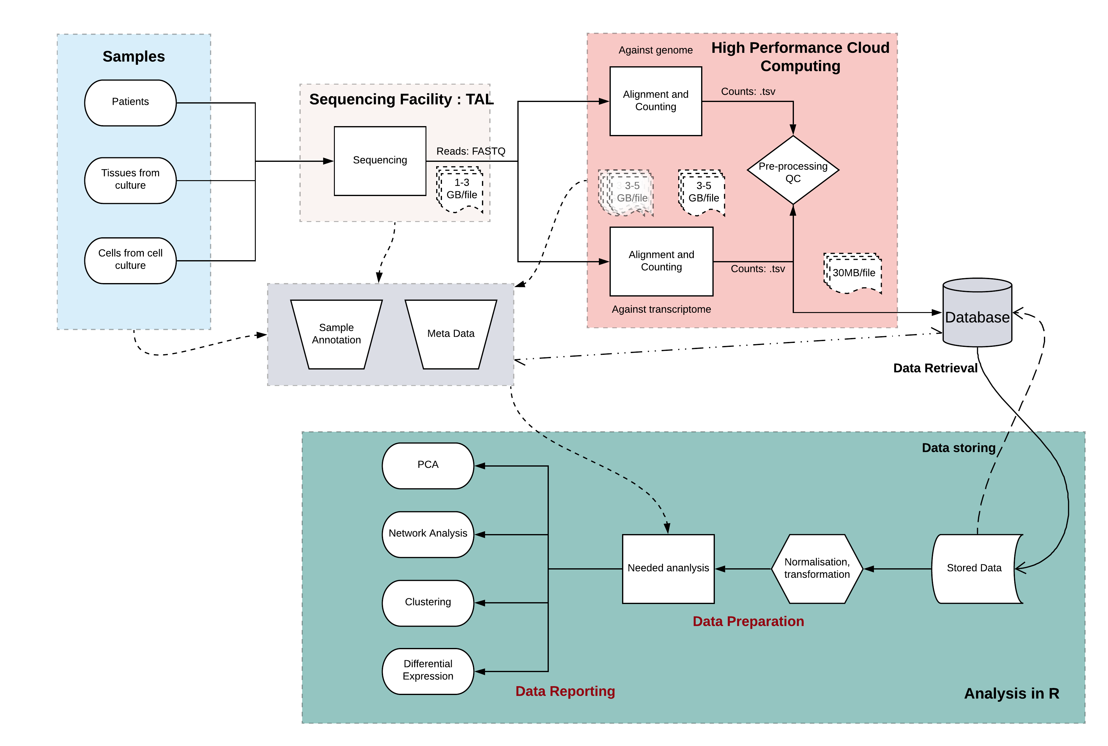
Figure 4.1: A General RNA-Seq Workflow. In general the source material of RNA-Seq is a sample either from patients, cell culture or tissues. After RNA extraction and optional enrichment, they get sequenced at a general sequencing (core) facility. This results in the generation of large files which are transferred to a HPC, where the first steps of alignment and abundance estimation is performed. Smaller count text files containing information on the transcripts and the quanitative amount of expression can then be easily stored in a local database for retrieval and further processing. The final steps of performing the required analysis specific for the question asked can be performed on any statistical environment (such as R) and visualized and deployed for publishing or internal use. Throughout this whole process it is vital to maintain a consistent and common, easy to use metadata collection system. Shapes and their meanings: cylinders (database), rhombus (decision points), rectangles (processes), oval (starting/ending points).

The average alignment for uniquely mapped reads is ~70% across all samples used in this study, while the number of reads assigned to specific genomic coordinates by featureCounts abundance estimation tool is on average ~60%. These fall within normal acceptable ranges. There were no excessive adaptor content or duplicated reads observed.

4.2 Exploring Potential Microbial Contamination using RNA-Seq Data

To explore the potential microbial contaminants amongst the sample data sets, a representative subset of samples were chosen, see Table 4.1, such that every category i.e., adult heart, fetal heart, CM, EHM is represented by one sample in the subset, chosen across different sequencing runs, different years and different projects. Human and non-human reads were separated and the latter were used as possible microbial read candidates. After a series of filtering, as explained in Section 3.4, the non-host, high-quality and unique reads were aligned against the reference genomes of bacteria and virus.

Table 4.1: Samples chosen for in-depth analysis

Sample	Sample Number	Project Accession
SRR1663123_GSM1554465	1	PRJNA268504
SRR6706796_GSM2991857	2	PRJNA433831
Sample_r733sCDICM3	3	In-House
p556sCM10-3-4	4	In-House
p637sDiff6CM	5	In-House
p722s3C190604	6	In-House
p786sC190924A	7	In-House

Table 4.2: Sample Read Statistics

		Human			Microbial
Sample Number	Total Reads	Primary	Multi-mapped	rRNA	Viral	Bacterial
1	35M	13M	16M	6M	20K	1K
2	20M	17M	1M	2M	24K	2K
3	51M	27M	20M	4M	190	949
4	53M	42M	10M	1M	70	5K
5	52M	31M	17M	3M	320	3K
6	51M	49M	60K	2M	966	14K
7	79M	36M	35M	8M	9K	3K

The general mapping statistics of the chosen samples can be seen in Figure 4.2A and tabulated in Table 4.2. Samples vary in terms of their sequencing depth (akin to the total reads column) and the proportion mapped to the human genome, which varies between 40% to 91% across samples.
A large variance is found in the number of viral/bacterial reads mapped per million human mapped reads, see Figure 4.2B.

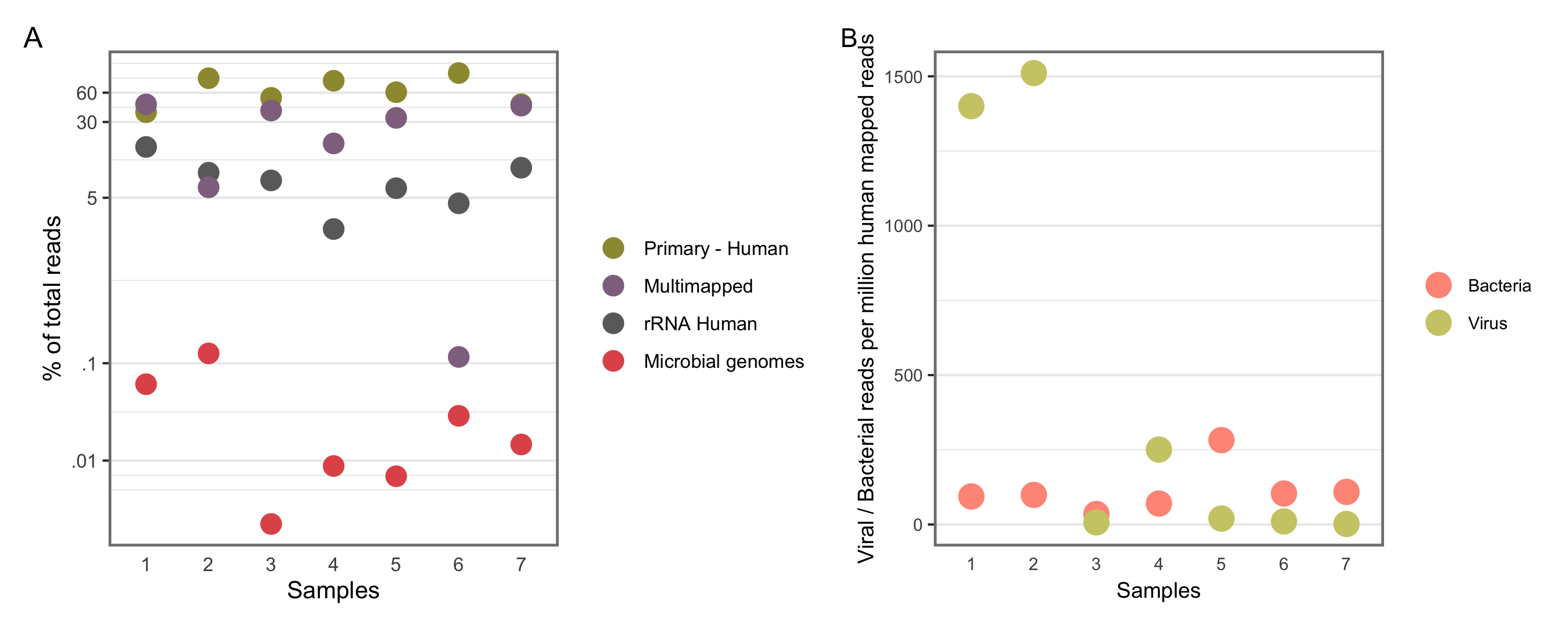
Figure 4.2: General Mapping Statistics. A shows samples and percentage of reads mapped to different groups. Y-aixs is in log scale to resolve low-expression reads. B shows shows separate bacterial and viral reads mapped per million human mapped reads per sample.

Absolute numbers of reads confidently assigned to different viral species across different samples is shown in Figure 4.3A. The same data is shown as relative abundance in Figure 4.3B. Samples 1 and 2 have a disproportionate number of reads, about 20,000 reads, mapped to a single viral genome — the col phage or phi-X174 (PhiX - NC_00 1422.1). Proteus phage is the second entity with high number of absolute reads assigned to it (~7000).

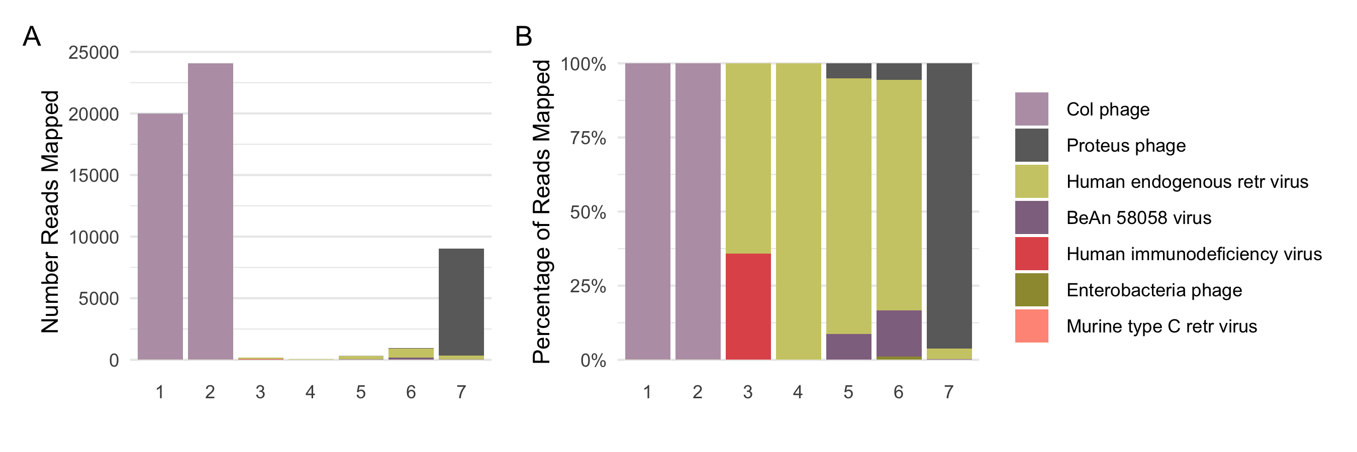
Figure 4.3: Possible viral contaminants. A shows the absolute number of reads confidently assigned to different viral species across different samples, while B represents them as relative abundances.

PhiX contaminants in samples 1 and 2 are most probably delibrately added as spike-in in illumina HISEQ platforms to increase nucleotide diversity. Samples 1 and 2 were sequenced on the HISEQ-2500⁶³ and HISEQ-4000⁶¹ platforms while all in-house samples were sequenced on HISEQ-2000³⁰ which has a separate, dedicated lane for the PhiX spike-in quality control to avoid PhiX reads to appear in the FASTQ files.³ Unusually high numbers of viral reads were seen in Sample 7, mostly that of Proteus phage VB_PmiS-Isfahan (NC_041925). Like other phage viruses, the Proteus phage also infects bacterial cells, specifically Proteus mirabilis a highly motile bacterium belonging to the Enterobacteriaceae family, which is the most common species responsible for catheter-associated urinary tract infections⁶⁵. No reads were confidently assigned to the Proteus genera of bacteria, however, proteus phage is considered to be highly lytic and there are several other bacteria belonging to the Proteus genera which are ubiquitously present on and in human guts which could be infected by the phage⁶⁶, hence making this assignment plausible. All other viruses detected were less 200 reads per sample except those that mapped to the HERVs. These are viral sequences that represent ancient viral infections that affected the primates’ germ line and became stably integrated into the host genome. This was an interesting find as ~ 8% of the human genome is said to be of viral origin, the HERVs. The reason behind its baseline expression in most of the adult tissues nor its role in different pathologies are not well defined^67–69.

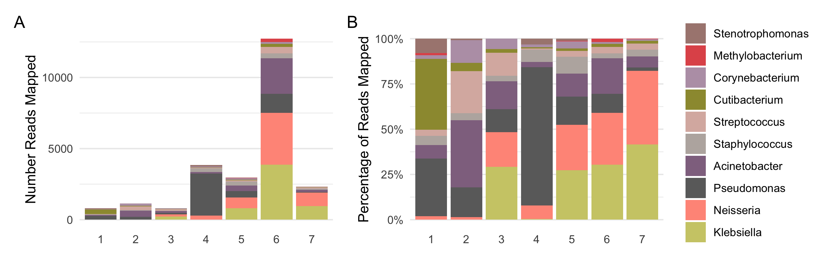
Figure 4.4: Possible bacterial contaminants at the Genus level. A shows the absolute number of reads confidently assigned to different bacterial genera across different samples, accounting for around 80 percent of all the reads assigned to bacteria, while B represents them as percentage proportions.

Unlike viral, the bacterial reads were analyzed at two levels, genus (Figure 4.4) and species (Figure 4.5). The 10 genera shown account for about ~80% of all reads mapped to bacteria while the 10 species shown account for about ~50% of all reads mapped. All samples except Sample 6, are within acceptable limits of bacterial reads/sample, less than 100 bacterial reads/million human mapped reads⁷⁰. Sample 6 has ~13500 reads in absolute numbers and approximately 250 bacterial reads/million human mapped reads, most of which are accounted for by 4 genera — Acinetobacter, Klebsiella, Neisseria, Pseudomonas. This is also reflected at the species level, where Klebsiella pneumoniae and Neisseria gonorrhoeae account for 57% of the entire bacterial contamination found in the sample while the rest is accounted for by 189 other species. Low levels of both these bacteria are also found in the other in-house samples. The presence of Cutibacterium acnes, Pseudomonas and Acinetobacter bacterial contamination has been well documented owing to their epidermal persence in the first case and to water associated presence, even ultra-purified, in the last two cases^71–73. While Klebsiella has been associated with pathologies, it is also a known opportunistic pathogen which is a normal part of the microbial flora of mucosal surfaces such as the mouth and throat and found ubiquitously in nature/environment⁷⁴. Likewise, although Neisseria gonorrhoeae is not a part of the normal flora, it could also present as benign/unnoticed infections of the mucosal surfaces urogenital tract, pharynx, and rectum, apart from causing a full-blown pathological disease⁷⁵. The discovery of bacterial reads in cell line data and the finding of different bacterial taxa in data from different sequencing runs/groups/labs supports the idea that a good portion of bacterial reads are possibly not derived from the specimens themselves.

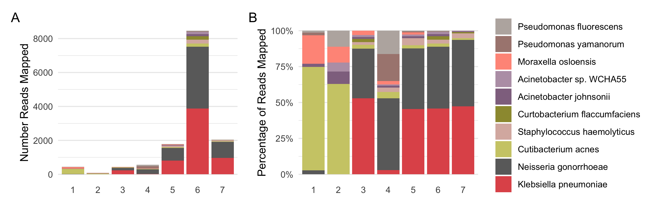
Figure 4.5: Possible bacterial contaminants at the species level. A shows the absolute number of reads confidently assigned to different bacterial species across different samples, accounting for around 50 percent of all the reads assigned to bacteria, while B represents them as percentage proportions.

The results from these 7 representative samples are in-line with papers published which looked at the microbial contamination in RNA-Seq samples in terms of their diversity and the range of proportions of microbial contamination differing between different samples. For instance, work by Strong et al⁷⁰, showed that Acinetobacter contributed to the highest number of reads. While the study by Park et al⁷⁶, also picked up a large number of samples having PhiX phage reads in them. All the samples assessed here have microbial reads less than 0.1% of total reads (including the first two samples if we account for the spike-in PhiX reads). This is considered very low and acceptible by other papers which have published on this topic⁷⁰, however, no rule/regulation stipulated by cGMP exists currently which deal with such non-standard exploration of microbial contamination in TEPs.
The samples also differed in their sequencing depths which would have influenced the extent to which metagenomic reads were picked up. This work is neither exhaustive nor confirmatory but since it has the possibility of working on already collected data, it could be a novel complementary and regulatory step that might one day be incorporated into a cGMP practice alongside other standard microbial detection techniques.

4.3 Global view of the transcriptomic data

Data from 68 samples were collected (20 iPSC-CMs, 17 EHM, 16 Fetal Heart samples, 15 Adult Heart Samples) across different studies as shown in Table 3.1. To examine global trends in gene expression levels, the normalized data across all samples were visualized using PCA (Figure 4.7). 72.4% of total variation in the dataset can be explained by the first 4 PCs and the cumulative percentage of the variances explained by the first eight PCs is shown as a scree plot (Figure 4.6A). The major source of variation in the data is correlated with the sample type and is captured by the first PC accounting for 42.9% of the variation in the data set, where the first PC effectively separates the sub-groups with an almost uni-directional progression from cardiomyocytes to EHMs to fetal heart tissue and adult heart subtypes, showing that this vector captures the increase in complexity of the tissue types (Figure 4.6B).

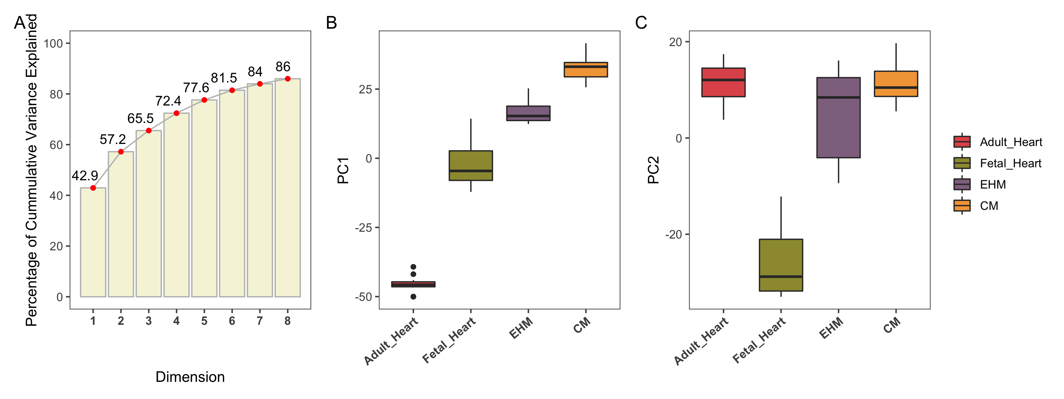
Figure 4.6: A shows the cummulative variance explained by the PCs. B and C show the different groups plotted against PC1 and PC2 respectively.

The second largest source of variation is captured by PC2 accounting for 14.3% of the total variance and separates the fetal heart samples from the rest of the sample types as shown by the ordering of sample types according to PC2, (see Figure 4.6C).

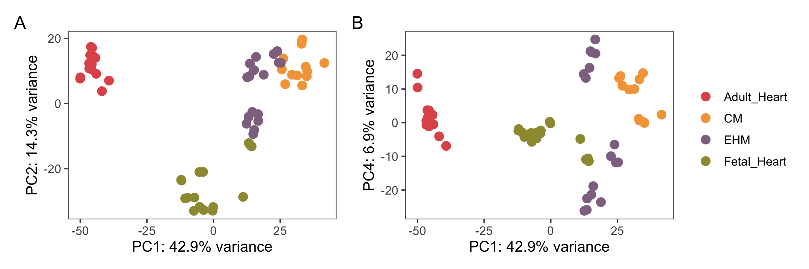
Figure 4.7: A and B show the PCA plots of all the samples againt PC1 and PC2/PC4. The samples are coloured based on their groups.

Cardiomyocyte samples which are >90% actinin+ in FACS are in-essence representative of a single cell type, while EHMs have the additional stromal cells. Apart from these two, fetal heart tissues also contain a variety of other cell types and sub-types including differentiated and differentiating cells along different lineages. The adult heart on the other hand is composed of not just cardiomyocytes and fibroblasts but also endothelial cells, immune cells, vascular smooth muscle cells and cells making up the conduction system. Fetal heart samples show relatively loose clustering compared to adult heart samples. This might be because the fetal samples were collected across different gestational periods, in the range of 9 weeks - 16 weeks (Figure 4.7A).

The EHM samples also show two semi-distinct clusters, corresponding to the two EHM sources — in-house and from the PRJNA362579 project. The source of this variation within the EHM samples appears to be strongly associated with PC4, see Figures 4.8 and 4.7B.

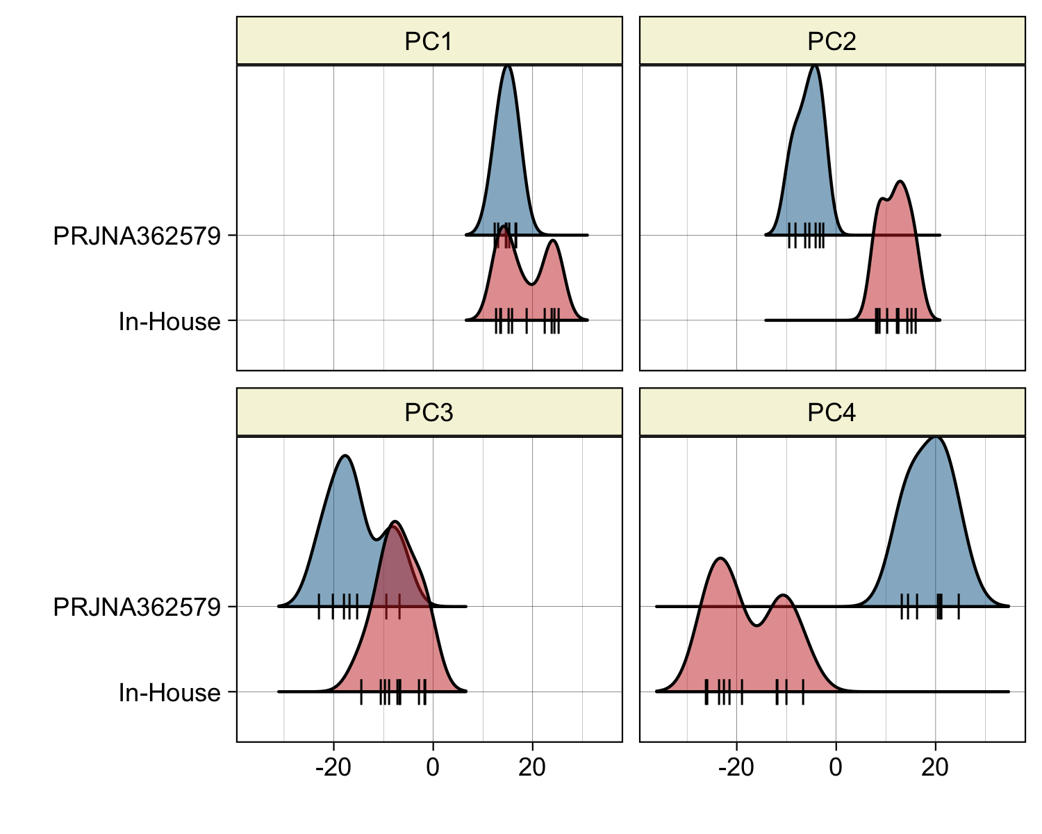
Figure 4.8: Separation of EHMs by the first 4 PCs. The two groups of EHMs and the varying degress of separation by different PCs, visualized by a density plot.

As explained in Section 1.5.1, the loading scores of genes can be explored further to look for possible meaningful explanations of the basis of separations of the clusters. The top 50 genes with the highest absolute loading values is tabulated for the first 4 PCs in Table 4.3.

Table 4.3: Top 50 Genes with the highest absolute loading in the first 4 PCs

Gene	PC	Gene	PC	Gene	PC	Gene	PC
GPR4	-0.033	ARHGAP33	-0.055	PLAT	-0.064	ANGPT2	-0.071
PDE2A	-0.033	PRRT2	-0.054	MMP14	-0.064	CLMP	-0.068
CD300LG	-0.033	MXD3	-0.054	ITIH3	-0.061	MEG8	-0.067
GIMAP1	-0.033	PIF1	-0.054	TNC	-0.060	F2RL2	-0.066
RAMP3	-0.033	KIF18B	-0.053	TGFBI	-0.059	DOCK10	-0.065
APOD	-0.033	CHTF18	-0.053	LIF	-0.059	SAMD9L	-0.062
SPAAR	-0.033	TROAP	-0.053	ENC1	-0.059	PI15	-0.062
RAI2	-0.033	HBG1	-0.052	LUM	-0.058	CTSK	-0.060
TMEM273	-0.033	SPTA1	-0.051	TIMP1	-0.057	PAMR1	-0.060
APOL3	-0.033	HBG2	-0.051	EFEMP1	-0.057	CCDC144B	-0.059
COL4A5	0.033	FAM95C	-0.051	FN1	-0.057	CLCA2	-0.059
SLC15A3	-0.033	EPB42	-0.051	SRPX2	-0.057	SAMD9	-0.058
SLC9A3R2	-0.033	HEMGN	-0.051	CFH	-0.056	CRB2	0.057
PRELP	-0.033	TMEM155	-0.051	RHOU	-0.056	TMEM119	-0.057
FABP4	-0.032	PKMYT1	-0.050	CCL2	-0.056	FAP	-0.057
GPX3	-0.032	YJEFN3	-0.050	IL1R1	-0.056	CITED4	0.057
RORC	-0.032	LENG8	-0.050	VGLL3	-0.056	PCDH18	-0.056
C1QA	-0.032	FOXM1	-0.050	SERPINE2	-0.056	RPL10P6	-0.055
DIRAS1	-0.032	ESPL1	-0.050	BNC2	-0.055	PUS7L	-0.055
TYROBP	-0.032	GRIA2	-0.049	NTM	-0.055	LAMA5	0.055
HSPB6	-0.032	EMC10	-0.049	EMILIN1	-0.055	POSTN	-0.054
FGR	-0.032	SLC4A1	-0.049	SULF1	-0.055	PRRX1	-0.054
SOX18	-0.032	DDX39B	-0.049	FXYD5	-0.055	NT5E	-0.054
CD79B	-0.032	PLK1	-0.049	ZNF280D	0.054	KCNJ2	-0.054
CRYM	-0.032	ALAS2	-0.049	GPRC5A	-0.054	TWIST2	-0.054
RPL3L	-0.032	CDT1	-0.049	CYP1B1	-0.054	ADGRG7	-0.053
FCN3	-0.032	MYBL2	-0.049	COL1A2	-0.054	ZNF528	-0.052
TMEM143	-0.032	MIR503HG	-0.049	RCN3	-0.054	TMSB4XP8	-0.052
PTGDR2	-0.032	CDCA3	-0.049	DKK1	-0.054	LPAR1	-0.052
HLF	-0.032	AGAP6	-0.049	F2RL1	-0.053	LINC01405	0.052
NDRG4	-0.032	TMCC2	-0.049	IGFBP3	-0.053	GABRA4	-0.052
ADGRE5	-0.032	PLEKHG4B	-0.048	NLRP2	-0.053	THBS2	-0.052
ACKR1	-0.032	HBM	-0.048	LOX	-0.052	PRRX2	-0.051
AQP7	-0.032	SOD2	0.048	ITGA11	-0.052	DPP4	-0.051
IGF2BP3	0.032	CDC42	0.048	ZNF680	0.052	AC096664.2	0.051
PLIN4	-0.032	FKBP2	-0.048	SPHKAP	0.052	CXCL10	-0.051
ICAM2	-0.032	CHTF8	-0.048	PTX3	-0.052	ZNF248	-0.051
CD38	-0.032	TTYH3	-0.048	NNMT	-0.052	AC016739.1	0.051
C1QB	-0.032	IGSF9	-0.048	HGF	-0.052	MYH6	0.051
CCM2L	-0.032	FAUP1	0.048	KRT17	-0.052	ZNF736	-0.051
ADAM15	-0.032	BHLHB9	-0.048	CTHRC1	-0.052	DDR2	-0.051
P2RY8	-0.032	NPIPB5	-0.048	MMP9	-0.052	MEG3	-0.050
TNFSF12	-0.032	AP002884.1	0.048	PTGS2	-0.052	FOXP4	0.050
CBX7	-0.032	AHSP	-0.048	ITGA8	-0.052	CLEC2B	-0.050
LGALS9	-0.032	GTSE1	-0.048	COL3A1	-0.052	MMP3	-0.050
DMTN	-0.032	TYMS	-0.048	CDKN2B	-0.051	AL161787.1	0.050
CLEC3B	-0.032	PRRG3	-0.047	SERPINB2	-0.051	CMKLR1	-0.049
SPI1	-0.032	COL6A6	-0.047	FBN1	-0.051	TMEM176B	-0.049
GIMAP7	-0.032	KIFC1	-0.047	BASP1	-0.051	CCN4	-0.049
ECHDC3	-0.032	E2F1	-0.047	VWC2	0.051	CNTFR	0.049

Genes in the first PC account for the majority of separation of adult heart samples from the rest. The genes discriminatory for the adult heart samples not only account for the mature adult cardiomycoytes but also for the other cell types primarily found in adult hearts biopsies like AQP7, possibly from the adipose tissue surrounding the heart⁷⁷ and APOD from aortic valves of the adult heart⁷⁸. These cell types would be atypical for bioengineered tissues and cultured cell and less common in the fetal heart samples. The current analysis pipeline, does not allow to quantify the relative closeness of the EHM groups to either fetal or adult phenotypes. Other biological and functional characterizations of the EHMs are necessary to complement the deconvolution approach.

4.3.1 Correlation amongst groups

Pearson correlation of cardiomyocytes, EHMs and fetal heart samples’ gene expression to that of adult heart based on the top 2000 genes with the highest absolute loadings in PC1 and PC2 was performed, to check for global similarity in expression patterns and is shown in Figure 4.9 A.2. These complement the observations from PCA and show that fetal heart samples have the highest similarity to adult heart samples (median ~0.6, with a notable range of 0.3 - 0.65), followed by EHMs (median ~0.45) and lastly by cardiomyocytes (median ~0.25). By choosing ~380 genes which are specifically detectable and enriched in the human heart, based on Human Protein Atlas data, the pearson correlation of the EHM and fetal samples becomes very comparable as shown in Figure 4.9 B.2. The median correlation of the EHM samples is even slightly higher than that of the fetal samples, which is in line with our estimation of the EHMs being comparable to (~13wk) fetal tissue⁷⁹. Gene expression across different sample types as per the curated gene list appears to be more consistent and comparable, as visualized in Figure 4.9 B.1 in comparison to Figure 4.9 A.1. The genes in the heatmaps are hierarchically clustered.

These results show that the separation in PC1 of all the different groups are possibly not due to differences in the expression of genes pertaining to CMs, as they all have a higher correlation when a subset of heart-specific genes was used. And this high correlation was lost when the top 2000 genes with the highest loading in PC1 was used, indicating that the highest variance amongst the groups is possibly not due to biological differences in their CMs expression profile.

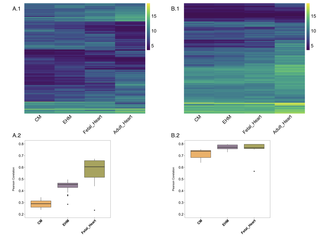
Figure 4.9: Correlation of samples. Heatmaps show VST normalized and group-wise clubbed data. A.1 shows the top 2000 genes with highest loading in PC1 and PC2. B.1 shows a heatmap drawn from a selection of ~380 genes based on Human Protein Atlas. In both the heatmaps each row represents a gene and each column represents the average of the sample group. A.2 and B.2 show the pearson correlation of the different groups to the adult heart samples based on either the top 2000 genes or the curated 380 genes.

4.3.2 Gene-level analysis

Despite crucial insights derived from the global view of samples, a view based on curated set of genes are also indispensible and remain one of the most common ways of comparing samples/groups using transcriptomic data. Here we selected four different groups of genes, covering an example of metabolic, structural and general gene lists as shown in Figure 4.10. Panel A is a selected representation of the 10 highest and most specifically expressed genes based on information from human protein atlas. Unsurprisingly the adult heart samples show the highest expression for these genes, except the Myom1 gene which has been recently found to be a putative marker for hPSC-induced cardiomyocytes’ maturity⁸⁰, which is almost equally expressed in all samples. Panel B consists of 22 genes associated with the sarcomere gene ontology term. Genes such as Myo3b, Capn3 have a lower expression in the adult heart samples as opposed to the others and are known to have distinct patterns of high expressions during the developmental timeline^81,82. Panel C is representative of the genes belonging to the oxidation-reduction pathway, while D is a gene list derived from the group’s prior publication which deduced that these 50 genes are differentially expressed and considered to be markers for cardiomyocytes. Notably, adult heart associated genes are generally highly expressed, followed by fetal and EHM samples. A few clear exceptions are genes such as Gpc3 which has a clear and marked role in vertebrate development⁸³, Myl4 and Myl7 are known to be expressed heavily by the developing heart^84–86, and Tnni3 which is known to be expressed under specific developmental conditions⁸⁷. This gives a snapshot of the approximate level of general (panel A and D), structural (panel B) and metabolic (panel C) maturation/status of the EHMs and cardiomyocytes at a transcript level in comparison to the fetal and adult heart samples. These observations are in line with previous results showing that cardiomyocytes in 2D are less mature than EHMs and at a population/tissue level the EHMs are similar to fetal heart samples.

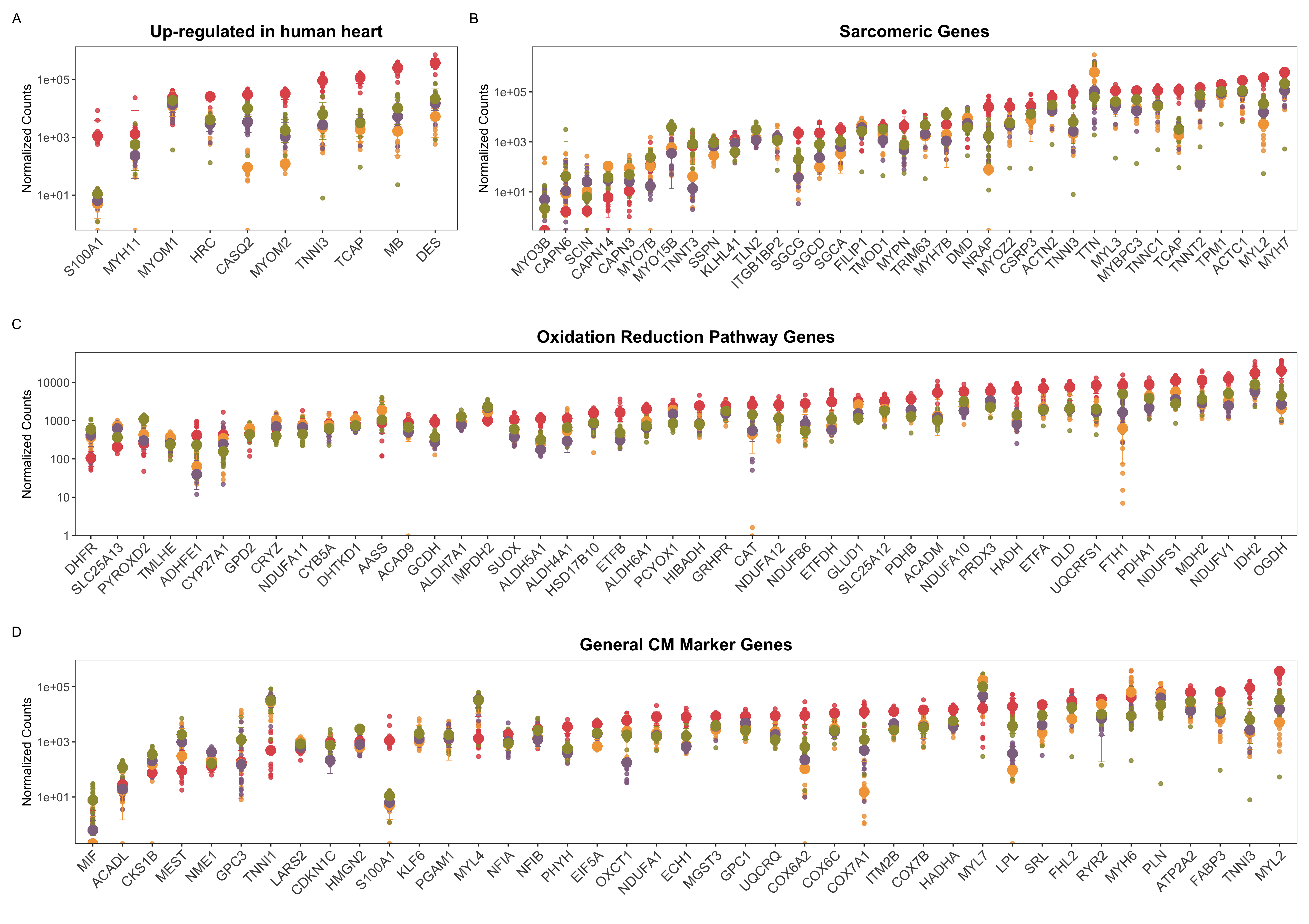
Figure 4.10: At individual gene level, the EHMs resemble the fetal heart expression levels. The graph shows normalized counts of different panels of gene sets. The bigger circles show the median of each group while the slightly transparent and smaller circles represent each sample for every gene. A shows the 10 highest and most specifically expressed genes as per human protein atlas. B contains 22 genes belonging to the sarcomere gene ontology term. C is representative of the genes belonging to the oxidation-reduction pathway and D is a gene list derived from the group’s prior publication which deduced that these 50 genes are differentially expressed and considered to be markers for cardiomyocytes

Exploring the data in the global context and at the gene-level did fortify pre-formed opinions but was of little help in the elucidation of the possible sub-populations within each sample. This was subsequently addressed by the deconvolution technique, as described below.

4.4 Deconvolution of Bulk CMs and EHMs RNA-Seq Data

Adult and fetal primary heart samples are natively heterogeneous with respect to cell composition, while bioengineered tissues consist of two main components and samples from targeted differentiations should contain one dominant cell type at beginning (iPSC) and end (CM) but go through stages with diverse transient cell populations in between. To rationalize and quantify the heterogeneity present within the in-house bulk samples, computational deconvolution was performed using a public single-cell reference sample⁵⁸. Based on the reference data, the last two time points sequenced during the differentiation of iPSCs to CMs are represented as Day 15 and Day 30 with two distinct sub-populations within each group. Day 15 is characterized by a non-contractile, fibroblast-like sub-group (denoted as d15:S1) and a contractile, cardiac-like/cCM sub-group (denoted as d15:S2). Similarly day 30 is characterized by two sub-groups — non-contractile cells (d30:S1) and cardiomyocytes/dCM (d30:S2) ), as tabulated in B of 4.11. Methodologically we followed a state of the art protocol, as described in Section 3.2, where d15 and d30 reference data were processed and used in CIBERSORTx to generate a signature-matrix, which was then used to deconvolve the bulk samples, whose results are shown as a percentage proportion bar graph in Figure 4.11A.

CMs samples are considered highly (>90% cardiomyocytes) pure while EHM samples were prepared from 70% cardiomyocytes and 30% stromal cells (~30%). To scale the CM samples for the 30% FBs in the EHM sample, a “virtual” cell type or comparability factor was added. The CM sample shows a larger proportion of d15:S1 phenotype-like cells (~57%) and a smaller proportion of d30:S1 (mature cardiomyocyte-like) cells as compared to EHMs, supporting the notion that CMs continue maturation when being exposed to the 3D EHM environment⁸⁸. The increase in duration of culture has been proposed to increase the maturity of the CMs, as also clearly evidenced by the deconvolution. It is also interesting to note that the deconvolution picked up the sparsity of non-cardiomyocyte-like cells in the CMs sample, only about ~9% of the sample is represented by the S2 sub-groups across both time-points, showing that the majority is composed by cardiomyocytes or cardiomyocytes-like cells. This clearly validates the current differentiation protocol. The difference in composition of the EHM samples from that of CMs is also captured efficiently as seen by the increase in proportion of S2 sub-groups (the non-contractile cells ) in the EHM samples.

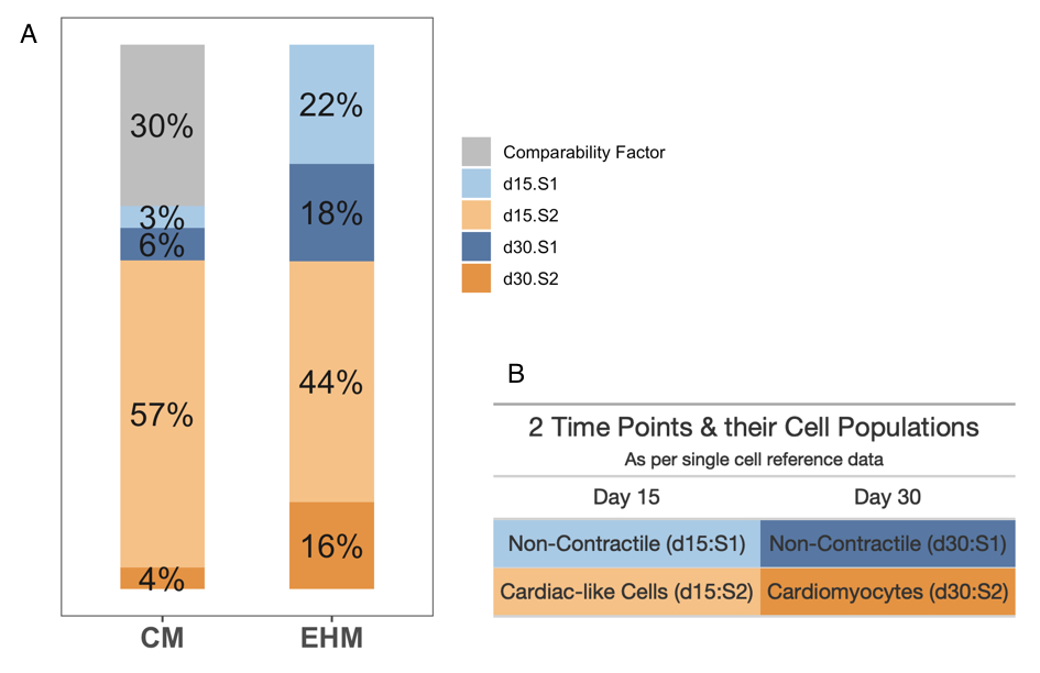
Figure 4.11: EHMs have a higher proportion of mature cardiomyocytes in comparison to CMs. A shows percentages of the various groups as per deconvolution, that are explained in B, along with a comparability factor added to the CM samples to allow for direct comparison of both CMs and EHMs.

As explained in Section 1.6, our group envisions to conduct clinical trials employing the usage of EHMs for treatment of heart failure. Given that CMs are a key component in the production of EHMs, it is vital that the batch-to-batch consistency is maintained. Currently four batches of CMs have been analyzed in Figure 4.12 post bulk-sequencing and subsequent deconvolution. The variation across samples within proportions sub-groups is not signficant (Figure 4.12A). Each sample and its corresponding deconvoluted putative sub-group percentages are shown in Figure 4.12B. It is evident that the majority of any CM sample is accounted for by the d15:S2 (immature cardiomyocyte) phenotype (~ 83%) which is in-line with the evidences from functional and structural experiments of the group. Across every differentiation run, the efficiency of differentiation is assessed using flow cytometric markers, and percentage of cells positive for Actinin 2 marker indicate the approximate amount of cells differentiated into cardiomyocytes. In particular, one among the four samples was observed to have low percentages of Actinin positive cells (~40%), which was suspected to be an error in handling of the flow cytometer than actual lack of purity. The results from deconvolution show that indeed all the samples have a large proportion of cardiomyocytes (mean ~87%), and the single, potential outlier from flow cytometry data was possibly erroneous.

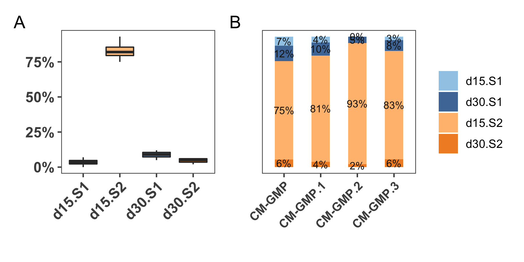
Figure 4.12: The GMP-CM samples are mostly consistent wrt subpopulations derived from deconvolution. A shows the box plots of the contribution of four sub groups across the four samples. B is a sample-wise representation of the sub-groups.

To see whether the difference observed between the two EHM sub-groups (in-house and from the project PRJNA362579) in PCA could be addressed using the deconvolution technique, a sample-level deconvolution was performed, as shown in Figure 4.13. It is seen that the EHM samples from project PRJNA362579 have a higher average percentage of mature-cardiomyocytes (d30:S2 ~ 23%) and more specifically, a sub group of the EHMs within it which the authors consider were more mature (~25%) due to differences in media supplementation (those labelled with MM medium). Those “mature” samples also have a higher combined percentage of d15:S1 and d30:S2 (i.e., all the cells committed to the cardiac lineage). The in-house samples show higher variation amongst the proportions of different sub-groups. This apparent consistency seen in the EHM samples from PRJNA362579, could be attributed to the fact that all these samples are from one study, primed for one hypothesis, while the in-house EHMs were sequenced across different years and different productions runs, along with changes in protocols. Yet, across the same cell-line or production batch, for instance the EHMs made from HES2 cell line, the consistency in putative sub populations are maintained.

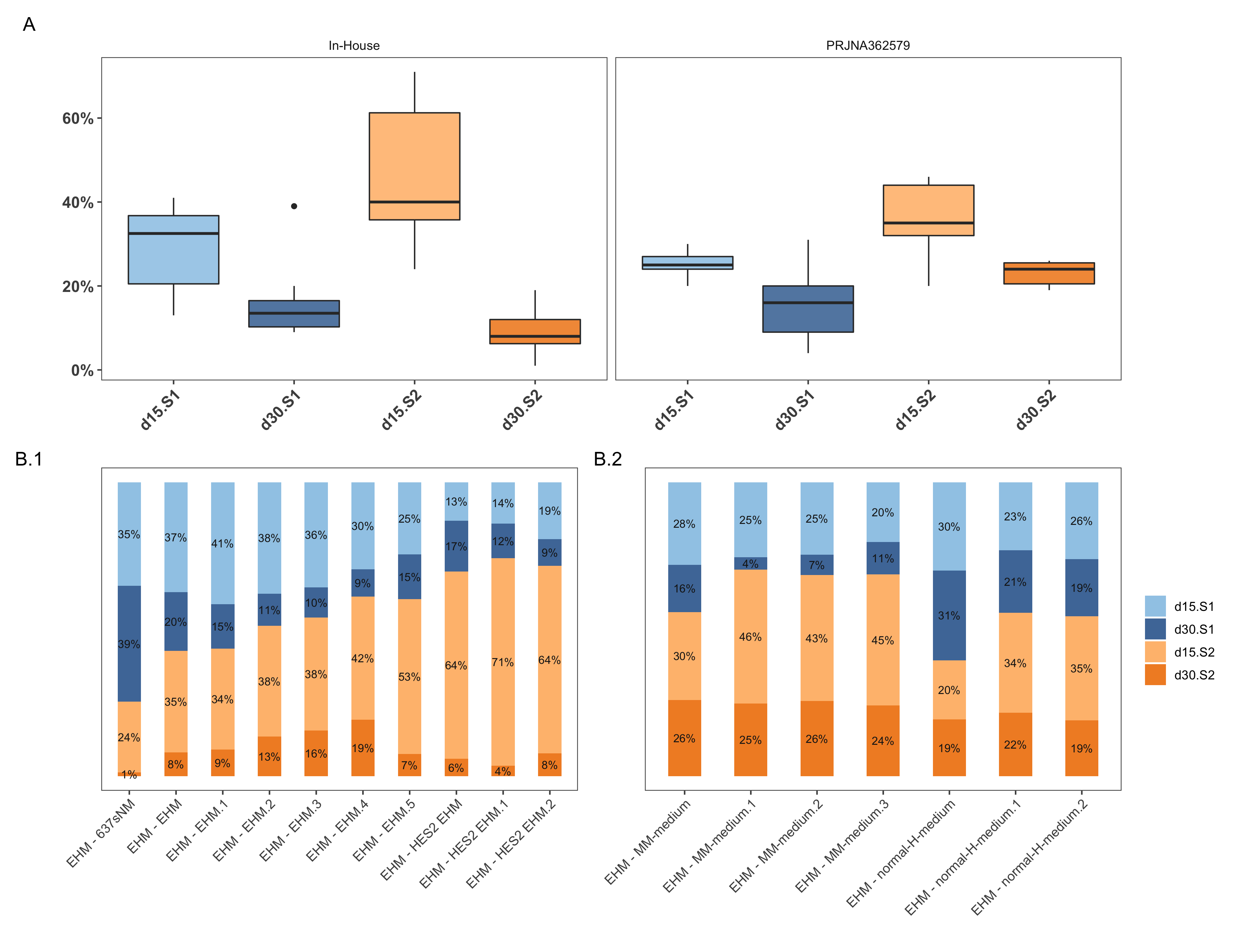
Figure 4.13: Differences in subpopulations amongst EHM samples. A shows the box-plots of percentage contributions of the various groups as per the source of the sample — in-house or from the PRJNA362579 project. B shows the corresponding sample-wise breakdown of the subpopulations in bulk data.

4.4.1 Limits of deconvolution

To address the reliability of the deconvolution technique, all sample groups and all samples within all groups were included (iPSCs, fibroblasts, CMs, EHMs, adult and fetal heart) and were deconvolved using the same reference dataset, as shown in Figure 4.15. Initially the validity of the deconvolution was evaluated by creating three different pseudo bulk samples, with known proportions of the sub-groups from the single cell data and these bulk samples were then deconvoluted, see Figure 4.14. Here we see that the deconvolution recaptiulates the true proportions, with an average RMSE of 0.1.

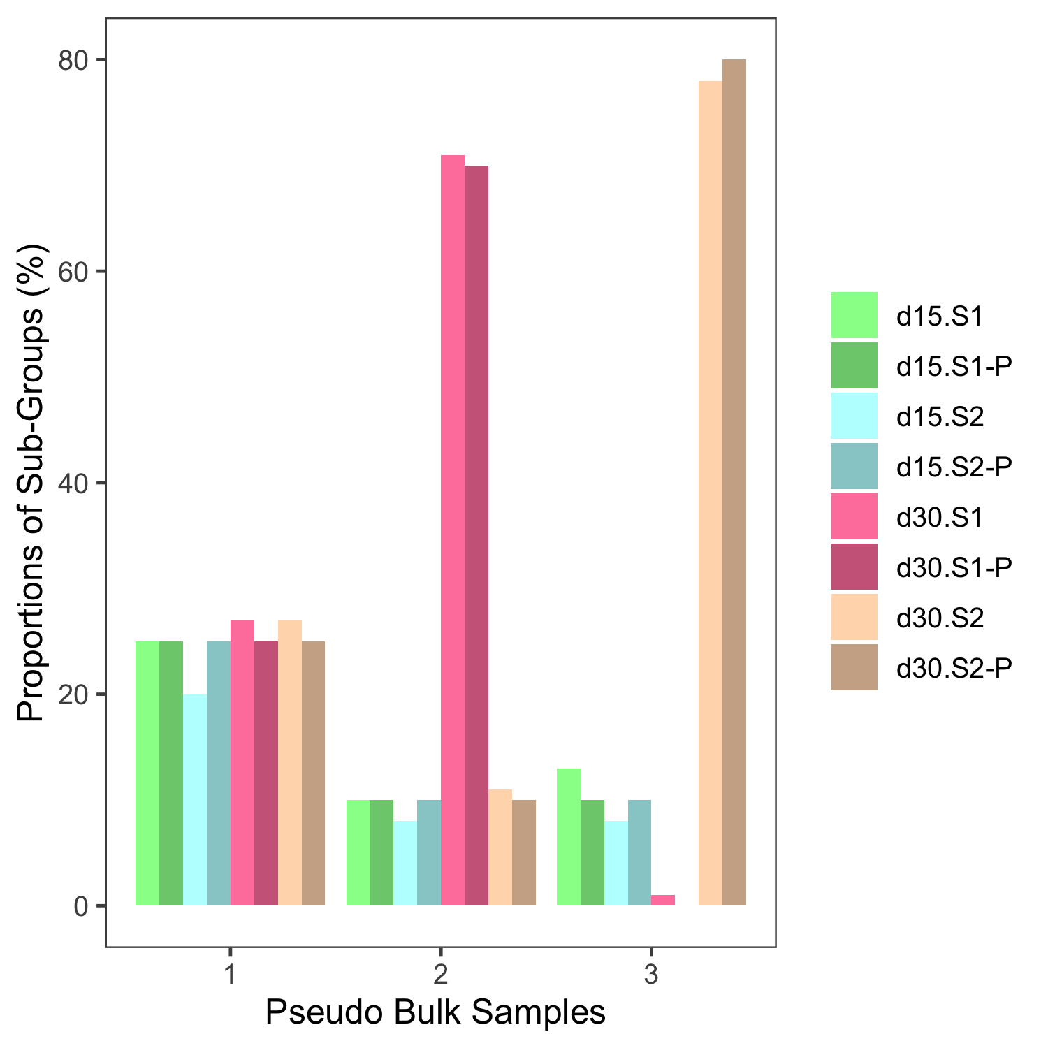
Figure 4.14: Estimating the validity of deconvolution. Three pseudobulk samples were created from the single cell reference data, the darker shade of the colours represent the known, true proportions of the four subgroups (denoted with a P). These samples were then deconvolved using CIBERSORTx and the resultant deconvolved estimated proportions are represented by the lighter shade bars adjacent to the true proportions.

On the other hand, when we use samples irrelevant or different from the reference data set, we can see that all the groups were deconvolved, yet, the reliability of these results varied widely. For instance, the root mean squared error (RMSE)⁴ of iPSCs and Fibroblasts are close to 1.0 while that of fetal heart group is around 0.3 (Figure 4.15B) . The correlation of the deconvolved results to the actual reference sample also had a large range, 0.19 for iPSC and 0.84 for the fetal heart. This shows the biggest limitation of such deconvolution techniques, and probably stands testimonial to the “garbage in, garbage out” situation, is the fact that deconvolution would work in any setting, however the usability of it depends on the relevance and similarity in composition of the cell types of the reference and the bulk data that needs to be deconvolved.

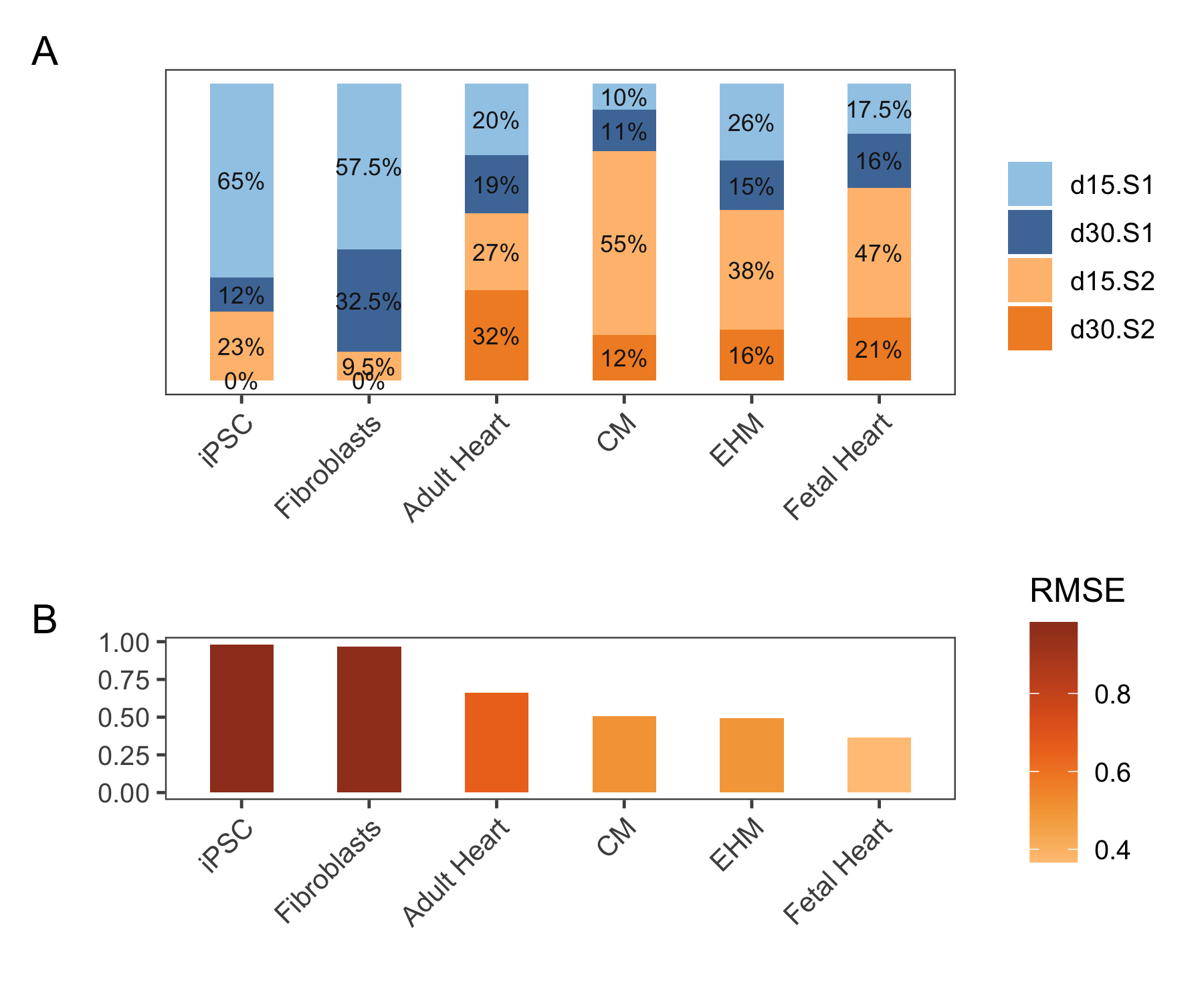
Figure 4.15: A shows the average deconvolution percentages of all groups to the four different subtypes. B shows the median RMSE of each group. Abbreviation: RMSE (root mean square error).

4.5 Basic characterisation of Rhesus Cardiomyocytes

To see where the cardiomyocytes produced from rhesus-iPSCs were placed in comparison to the human-iPSCs cardiomyocytes, the RH-CM samples were sequenced and processed. These rhesus cardiomyocytes were produced to produce EHM patches which were then transferred to a heart failure model of non-primate rhesus models. After retaining only the 1:1 orthologous genes and accounting for variations in gene lengths, the resultant samples were visualized in a basic PCA plot (Figure 4.16). All the samples are separated according to the cell type, starting with the first PC separating stromal cells and cardiomyocytes while the second PC separating iPSCs from the rest. Here, the human cardiomyocytes and rhesus cardiomyocytes (denoted as RH-CM) cluster together, and further analysis using DE showed that most of these differences were due to non-cardiac factors such as differences in signalling pathways and neuronal components possibly due to the fact that the rhesus cardiomyocytes were induced using the same protocol used for human cells which does not account for the differences in intricacies in the signalling pathways between the two.

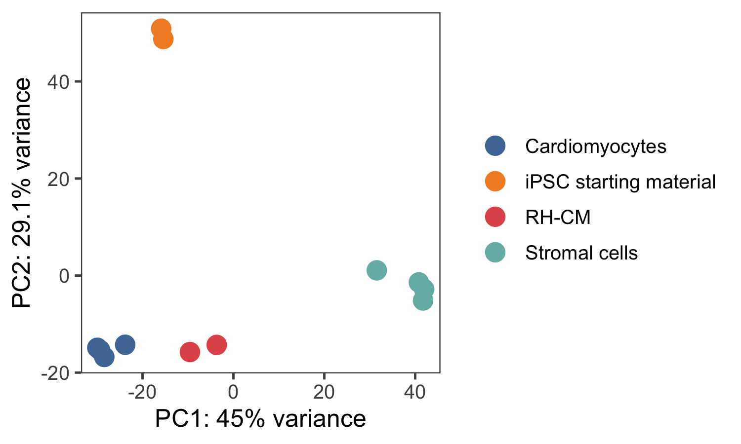
Figure 4.16: PCA of different samples, iPSCs, fibroblasts, human CMs and rh-CMs show that the rhesus CMs cluster with the human CMs.

References

30. Tiburcy, M. et al. Defined Engineered Human Myocardium with Advanced Maturation for Applications in Heart Failure Modelling and Repair. Circulation 135, 1832–1847 (2017).

58. Friedman, C. E. et al. Single-Cell Transcriptomic Analysis of Cardiac Differentiation from Human PSCs Reveals HOPX-Dependent Cardiomyocyte Maturation. Cell Stem Cell 23, 586–598.e8 (2018).

61. Pavlovic, B. J., Blake, L. E., Roux, J., Chavarria, C. & Gilad, Y. A Comparative Assessment of Human and Chimpanzee iPSC-derived Cardiomyocytes with Primary Heart Tissues. Scientific Reports 8, 15312 (2018).

63. Yan, L. et al. Epigenomic Landscape of Human Fetal Brain, Heart, and Liver. The Journal of Biological Chemistry 291, 4386–4398 (2016).

65. Schaffer, J. N. & Pearson, M. M. Proteus mirabilis and Urinary Tract Infections. Microbiology spectrum 3, (2015).

66. Drzewiecka, D. Significance and Roles of Proteus spp. Bacteria in Natural Environments. Microbial Ecology 72, 741–758 (2016).

67. Grandi, N. & Tramontano, E. Human Endogenous Retroviruses Are Ancient Acquired Elements Still Shaping Innate Immune Responses. Frontiers in Immunology 9, (2018).

69. Nelson, P. N. et al. Demystified . . . Human endogenous retroviruses. Molecular Pathology 56, 11–18 (2003).

70. Strong, M. J. et al. Microbial Contamination in Next Generation Sequencing: Implications for Sequence-Based Analysis of Clinical Samples. PLoS Pathogens 10, (2014).

71. K’eki, Z., Gr’ebner, K., Bohus, V., M’arialigeti, K. & T’oth, E. M. Application of special oligotrophic media for cultivation of bacterial communities originated from ultrapure water. Acta Microbiologica Et Immunologica Hungarica 60, 345–357 (2013).

73. Salter, S. J. et al. Reagent and laboratory contamination can critically impact sequence-based microbiome analyses. BMC Biology 12, 87 (2014).

74. Bengoechea, J. A. & Sa Pessoa, J. Klebsiella pneumoniae infection biology: Living to counteract host defences. FEMS Microbiology Reviews 43, 123–144 (2019).

75. Escobar, A., Rodas, P. I. & Acuña-Castillo, C. MacrophageNeisseria gonorrhoeae Interactions: A Better Understanding of Pathogen Mechanisms of Immunomodulation. Frontiers in Immunology 9, (2018).

76. Park, S.-J. et al. A systematic sequencing-based approach for microbial contaminant detection and functional inference. BMC Biology 17, 72 (2019).

77. Madeira, A., Camps, M., Zorzano, A., Moura, T. F. & Soveral, G. Biophysical Assessment of Human Aquaporin-7 as a Water and Glycerol Channel in 3T3-L1 Adipocytes. PLOS ONE 8, e83442 (2013).

78. Nordquist, E., LaHaye, S., Nagel, C. & Lincoln, J. Postnatal and Adult Aortic Heart Valves Have Distinctive Transcriptional Profiles Associated With Valve Tissue Growth and Maintenance Respectively. Frontiers in Cardiovascular Medicine 5, (2018).

79. Tiburcy Malte et al. Defined Engineered Human Myocardium With Advanced Maturation for Applications in Heart Failure Modeling and Repair. Circulation 135, 1832–1847 (2017).

80. Cai Wenxuan et al. An Unbiased Proteomics Method to Assess the Maturation of Human Pluripotent Stem CellDerived Cardiomyocytes. Circulation Research 125, 936–953 (2019).

81. Fougerousse, F. et al. Calpain3 expression during human cardiogenesis. Neuromuscular disorders: NMD 10, 251–256 (2000).

82. Liu Qing et al. Genome-Wide Temporal Profiling of Transcriptome and Open Chromatin of Early Cardiomyocyte Differentiation Derived From hiPSCs and hESCs. Circulation Research 121, 376–391 (2017).

83. Ng, A. et al. Loss of glypican-3 Function Causes Growth Factor-dependent Defects in Cardiac and Coronary Vascular Development. Developmental biology 335, 208–215 (2009).

84. Pawlak, M. et al. Dynamics of cardiomyocyte transcriptome and chromatin landscape demarcates key events of heart development. Genome Research 29, 506–519 (2019).

86. Wang, T. Y. et al. Human cardiac myosin light chain 4 (MYL4) mosaic expression patterns vary by sex. Scientific Reports 9, 1–7 (2019).

87. Sheng, J.-J. & Jin, J.-P. TNNI1, TNNI2 and TNNI3: Evolution, Regulation, and Protein Structure-Function Relationships. Gene 576, 385–394 (2016).

88. Machiraju, P. & Greenway, S. C. Current methods for the maturation of induced pluripotent stem cell-derived cardiomyocytes. World Journal of Stem Cells 11, 33–43 (2019).

---

3. Information obtained from Oregon State University’s Core facilities website Link.↩

4. The RMSE is the square root of the variance of the residuals. It indicates the absolute fit of the model to the data — how close the observed data points are to the model’s predicted values. Lower values of RMSE indicate better fit.↩